Drafting and publishing reproducible scientific articles with R Markdown
Source:vignettes/reproducr.Rmd
reproducr.RmdThe basics
Introduction
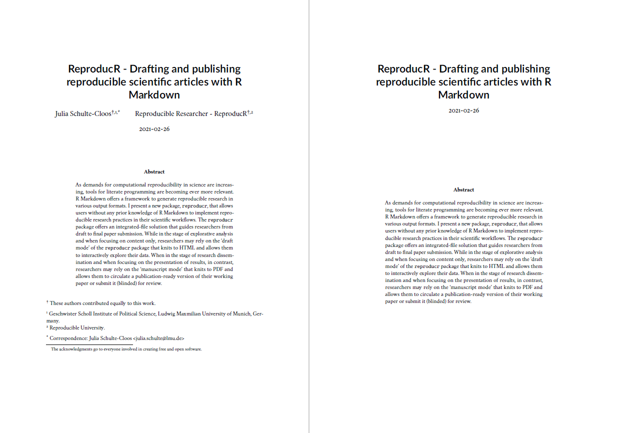
As demands for computational reproducibility in science are increasing, tools for literate programming are becoming ever more relevant. R Markdown offers a framework to generate reproducible research in various output formats.
The reproducr package allows users without any prior knowledge of R Markdown to implement reproducible research practices in their scientific workflows. The reproducr package offers an integrated-file solution that guides researchers from draft to final paper submission.
You enjoy full flexibility to knit your document to a polished and well-formatted HTML that includes all your explorative analysis and the interactive elements of your research output. This feature is particularly useful while drafting a research paper or when writing up blog posts to communicate your results to a wider audience. At the same time, you can knit your document to a polished and submission-ready PDF manuscript which is optimised for scholarly use and can optionally be blinded for review.
When writing your paper and your code, simply wrap the parts of the paper that are exclusive to one output format with three colons ::: {.not-in-format .latex} and the respective part of the document will not be included in \(\LaTeX{}\) output. You can also make the code evaluation conditional on the output format by asking knitr to conditionally evaluate your code only when the output is HTML: eval=knitr::is_html_output().
Markdown syntax
Markdown is so popular because it is a human-readable syntax, which is incredibly straightforward to understand. You can add bold content by adding two asterisks around the word that you want to emphasise (**bold**), whereas text will be shown in italics by wrapping it in simple asterisks (*italics*). You introduce sections with a hashtag (# A section or ## A level-two section).
If you do not specify a section label, Pandoc will automatically assign a label based on the title of your header and an algorithm that converts all alphabetic characters to lower case, removes all non-alphanumeric characters other than underscores, hyphens and periods and replaces spaces with hyphens. The section called ## My exciting introduction!, for instance, will be labelled as my-exciting-introduction. For more details, see the Pandoc manual. If you wish to add a manual label to a header, you may add {#mylabel} to the end of the section header.
Links are included by wrapping the text in square brackets and including the URL in parentheses, e.g. a [link](/url). You can include lists with simple bullet points or numbers for a numbered list. You can also include footnotes in your text, e.g. ^[An important footnote.].
- first item
- second item
- third item
Code chunks
The key to literate programming are code chunks, which are embedded in your manuscript written in Markdown. While the default programming engine used in R Markdown documents is the statistical programming software R, a number of other engines are also supported. A code chunk opens with three backticks (```{r my-code-chunk-label}) and closes with three backticks (```). You can easily insert a code chunk using the keyboard shortcut Ctlr+Alt+I in the R Studio IDE. It is a good practice to add a label for each code chunk, using only letters, numbers, or dashes while avoiding any other special characters.
Note that each code chunk needs to have a unique name within your document.
The reproducr package displays all code by default (folded in the HTML output) while it does not display any code by default in the PDF output. If you would like to change this behavior, you can change the respective global knitr chunk option, for instance, by: knitr::opts_chunk$set(echo = FALSE), which would hide all code – even in the HTML output.
YAML header
In the YAML header of your document, you can specify metadata that are central to your scientific manuscript, like the title of your document, the names of the authors, their affiliations, or the abstract of the manuscript. Most of these variables have their dedicated metadata field, e.g. title: 'An exciting new study in the field of xyz.'. The YAML header starts and ends with three dashes ---, like this:
---
documentclass: article
title: 'An exciting new study in the field of xyz.'
author:
  - name: "Reproducible Researcher"
    institute: [reprouniversity]
    correspondence: true
    email: reproducible.researcher@reprouniversity.edu
date: "2021-03-03"
institute:
  - reprouniversity:
      name: Reproducible University.
output:
  reproducr::reproducr_manuscript:
    blinded: false
---
You need to pay attention to indentation when modifying any parts of the YAML header. Currently, the RStudio IDE does not include a YAML linter, but you can either use any online YAML linter to check the validity of your YAML code, rely on a python-based application, or work with a different IDE, e.g. PyCharm together with its R Markdown Plugin.
R Markdown also stores the values of the metadata in an object metadata. Therefore, you can also include any information in the literate programming of your document, for instance, to print out the title of your document with rmarkdown::metadata$title (R Markdown will compile this to show the title of your document.
Explorative stage
Explorative data analysis
In the stage of explorative data analysis, you may want to dynamically explore your data and research output in interactive tables, graphs, or maps.
The reproducr package allows you to include any HTML-based interactive elements in your reproducr::reproducr_draft output.
Interactive graphs
In the explorative stage of data analysis, you can rely on interactive graphs, e.g., with the ggiraph package, which allows us to add tooltips, animations, or even JavaScript actions to existing ggplot objects.
Tip: Create your static ggplot object in one code chunk and specify a chunk option to include this chunk only if your output is \(\LaTeX{}\) with include=knitr::is_latex_output().
In a second code chunk, you can then further augment your ggplot with ggiraph without having to repeat the ggplot code. For this chunk, in turn, simply specify the chunk option include=knitr::is_html_output().
pacman::p_load(ggiraph)

# add interactive tooltip to the scatter_mass_flipper (static) ggplot object
scatter_mass_flipper <- scatter_mass_flipper +
  geom_point_interactive(
    aes(tooltip = paste0("<b>Flipper Length: </b>",
                         round(flipper_length_mm,
                               digits=2)
                         )
        ),
    size=1)

girafe(ggobj = scatter_mass_flipper,
       width_svg=7,
       height_svg=3.5)
Body mass and flipper length of penguins (interactive plot).
Interactive maps
In the HTML output of the reproducr package, we can also include any other interactive content, e.g., a leaflet map.
pacman::p_load(leaflet)

leaflet(height=200,
        width=500) %>%
  addTiles() %>%
  addMarkers(lat=48.15002,
             lng=11.59428,
             popup="LMU Munich") %>%
  setView(lat=48.15002,
          lng=11.59428, zoom=10)
Date stamps
The reproducr package allows you to knit your document to an output file that contains a date stamp at the end of the document’s name.
---
knit: reproducr::knit_with_datestamp
output:
  reproducr::reproducr_manuscript:
    blinded: false
  reproducr::reproducr_draft
---
The name of your .Rmd file will remain unchanged, allowing you to easily keep track of any changes in your file with version control tools like Git.
Dissemination stage
Layout and fonts
Layout
\(\LaTeX{}\) does respect the layout and aesthetics of documents – and you should keep doing so, too, when knitting to a \(\LaTeX{}\) based PDF document via the reproducr::reproducr_manuscript output format.
Make sure to specify a documentclass in your YAML header. Otherwise, R Markdown enforces page margins of 1 inch, which is hardly optimal for readability.
---
documentclass: 'scrartcl'
linestretch: 1.25
indent: true
output:
  reproducr::reproducr_manuscript:
    keep_tex: yes
---
Integration of fonts
The reproducr manuscript relies on the Cochineal font family as implemented in the cochineal \(\LaTeX{}\) package and the newtxmath \(\LaTeX{}\) package loaded with the cochineal option for optimal corresponding math support.
To integrate the fonts in the graphs of your document, e.g. created with ggplot, the reproducr package relies on the showtext package and the ragg_png graphic device of the ragg package.
Tip: create two chunks that specify a global ggplot font and evaluate each of them conditionally only when the output for \(\LaTeX{}\) or HTML output by adding the knitr chunk option eval=knitr::is_latex_output() or eval=knitr::is_html_output().
The code below shows how you can load Google Crimson Text font, matching the Cochineal font family used in the reproducr package for PDF output and store it as ggplot_font. In a second chunk, you would do the same, but instead specify a font optimised for HTML output, which you would only evaluate if the output format is HTML.
pacman::p_load(ggplot2,
               showtext)


## add a font from google fonts
font_add_google(
  name = "Crimson Text",
  family = "Crimson Text"
  )
ggplot_font = "Crimson Text"
## set-up the ggplot default theme of the document
ggplot2::theme_set(
  theme_bw() +
    theme(text = element_text(family = ggplot_font)) +
    theme(
      plot.title = element_text(
        hjust = 0.5
        ),
      plot.subtitle = element_text(
        hjust = 0.5
        )
      )
)
Blinded manuscript
The reproducr package allows you to blind your manuscript and exclude any author information, which may be necessary when you submit your research article for review.
---
output:
  reproducr::reproducr_manuscript:
    blinded: false
---
Bibliography and Reference Management
References for main body and appendix
The reproducr package allows you to include two separate bibliographies, one after the main body of the manuscript including all references of the main article and another bibliography at the end of the appendix, including only all of those references included in the appendix. This feature is currently not enabled in the standard R Markdown output formats.
In the YAML header, specify the section-refs-bibliography variable to refer to your .bib file.
---
output:
  reproducr::reproducr_manuscript:
    blinded: false
#Management of different bibliographies in PDF Manuscript
reference-section-title: 'References'
section-refs-level: 1
section-refs-bibliography: 'literature.bib'
# Management of Citation Styles
csl: 'https://bit.ly/3khj0ZL'
---
Note that the csl field does not need to link to a .csl file stored on your local machine, but can also link to a URL that contains the most recent version of the respective citation language style (CSL) that you use. In the example above, the link directs to a csl stored in the official repository for Citation Style Language (CSL) citation styles.
Because R Markdown ‘forces’ the Pandoc --citeproc option when you still specify the usual bibliography field in the YAML header and hard-codes this option as the last command into the Pandoc command line, currently, you need to comment any normal bibliography field out of the YAML header if you knit to reproducr::reproducr_manuscript and would like to include two separate bibliographies in your document. Future releases of this package will find a work-around for this somewhat unclean R Markdown behavior. Comments and contributions are welcome!
Indentation of the references
The Pandoc \(\LaTeX{}\) default template sets the hanging indent of the references to 1.5em in case your .csl file features a hanging indent. The Pandoc default .csl file is chicago-author-date, which has a hanging-indent style. There are also non-hanging-indent styles like harvard-cite-them-right.csl.
Default citation style language (CSL) and custom CSL files
The YAML metadata field csl can link to a file stored on your local machine or to a URL, which will be fetched via HTTP. If the file you specify on your computer cannot be found relative to the working directory, Pandoc will first look for it in the resource path (the default resource path is set to be the working directory) and finally in the csl subdirectory of the pandoc user data directory.
Remember that if your document specifies a csl style, Pandoc will convert Markdown references, i.e., @palmerdata.2020, to ‘hard-coded’ text and a hyperlink to the reference section in your document.
